

IVF_*,IVF_HNSW_*) and method of quantization (PQ,RQ,SQ).
IVF_PQ— Inverted File index with Product Quantization (default). See the vector indexing guide forIVF_PQexamples.IVF_SQ— Inverted File index with Scalar Quantization. This is available in Python and Rust; TypeScript does not currently exposeIvfSq.IVF_RQ— Inverted File index with RaBitQ quantization (binary, 1 bit per dimension). Requires vector dimensions divisible by8. See below for details.IVF_HNSW_SQ— IVF partitions with an HNSW graph per partition plus Scalar Quantization. Strong recall/latency/size trade-off for most workloads.IVF_HNSW_PQ— IVF partitions with an HNSW graph per partition plus Product Quantization. Prefer when PQ-level compression matters and you still want HNSW-style in-partition search.
IVF_PQ works well in many cases, but RaBitQ (IVF_RQ) allows for more aggressive compression.
See the “Choose the Right Index” table for further discussion.
todo decide what to do here vv
Use the same distance metric when training and querying the index. For IVF-based indexes, num_partitions controls the number of groups and sample_rate controls how many training vectors are sampled per partition, so the training sample is roughly sample_rate * num_partitions.
##Quantization Techniques
Product Quantization
Quantization is a compression technique used to speed up search by reducing the dimensionality of an embedding. Product quantization (PQ) first projects each large, high-dimensional vector into equal-sized subvectors. Each subvector is assigned a “reproduction value” that maps to the nearest centroid of points for that subvector. The reproduction values are then assigned to a codebook using unique IDs, which can be used to reconstruct the original vector.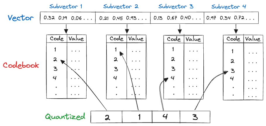
Original storage:
128 × 32 = 4096 bits.
Quantized storage: 4 × 8 = 32 bits.In this example, quantization achieves a 128x reduction in the memory requirement of each indexed vector.RaBitQ quantization
RaBitQ is a binary quantization method that represents each normalized embedding using 1 bit per dimension, plus a couple of small corrective scalars. In practice, a 1,024-dimensionalfloat32 vector that would normally take 4 KB can be compressed to roughly a few hundred bytes with RaBitQ, while still maintaining reasonable recall.
How RaBitQ works
- Embeddings are grouped around centroids (as in other IVF indexes).
- Each residual vector is normalized and mapped to the nearest vertex of a randomly rotated hypercube on the unit sphere.
- The sign pattern of that vector is stored as bits (1 bit per dimension).
- Two small corrective factors are stored:
- The distance from the original vector to its centroid
- The dot product between the normalized vector and its quantized version
IVF_PQ, RaBitQ:
- Avoids training expensive PQ codebooks
- Builds indexes faster and handles updates more easily
- Maintains or improves recall at high dimensionality under the same storage budget
Using RaBitQ
You can create an RaBitQ-backed vector index by settingindex_type="IVF_RQ" when calling create_index.
When using
IVF_RQ, the dimension of vectors must be a multiple of 8.num_bits controls how many bits per dimension are used:
1 bit is the classic RaBitQ setting. You can set it to 2, 4, or 8 bits to improve fidelity for better precision or recall — the main trade-off is additional storage for the extra bits per dimension, with only a modest increase in query-time compute.
It’s also possible to tune the number of IVF partitions in IVF_RQ, similar to how you would do in IVF_PQ.
###SQ (todo?)
API Reference
The full list of parameters to the algorithm are listed below.distance_type: Literal[“l2”, “cosine”, “dot”], defaults to “l2”
The distance metric to use for similarity comparison. Choose “l2” for Euclidean, “cosine” for cosine similarity, or “dot” for dot product.num_partitions: Optional[int], defaults to None
Number of IVF partitions (affects index build time and query accuracy). More partitions can improve recall but may increase build time. When unset, LanceDB chooses roughly the square root of the row count.num_bits: int, defaults to 1
Bits per dimension for quantization (1 is standard RaBitQ). Higher values improve fidelity, mainly at the cost of additional storage.max_iterations: int, defaults to 50
Maximum number of iterations for training the quantizer. Increase for larger datasets or to improve quantization quality.sample_rate: int, defaults to 256
Number of samples per partition during training. Higher values may improve accuracy but increase training time.target_partition_size: Optional[int], defaults to None
Target number of vectors per partition. Adjust to control partition granularity and memory usage. Ifnum_partitionsis also set,num_partitionstakes precedence.