Indexing Data

An index is a data structure that facilitates efficient scans and lookups on the embeddings of a given dataset. LanceDB provides a comprehensive suite of indexes to optimize query performance across diverse workloads:

Vector Index: Optimized for searching high-dimensional data (like images, audio, or text embeddings) by efficiently finding the most similar vectors
Full-Text Search Index: Enables fast keyword-based searches by indexing words and phrases
Scalar Index: Accelerates filtering and sorting of structured numeric or categorical data (e.g., timestamps, prices)

Scalar indices serve as a foundational optimization layer, accelerating filtering across diverse search workloads. They can be combined with:

Vector search (prefilter or post-filter results using metadata)
Full-text search (combining keyword matching with structured filters)
SQL scans (optimizing WHERE clauses on scalar columns)
Key-value lookups (enabling rapid primary key-based retrievals)

Supported Index Types

LanceDB provides a comprehensive suite of indexes for different data types and use cases:

Index	Use Case	Description
`IVF` (Vector)	Large-scale vector search with configurable accuracy/speed trade-offs. Supports binary vectors with hamming distance.	Inverted File Index—a partition-based approximate nearest neighbor algorithm that groups similar vectors into partitions for efficient search. Distance metrics: $\ell_2$ `cosine` `dot` `hamming` Quantizations: `None/Flat` `PQ` `SQ` `RQ`
`IVF_HNSW` (Vector)	Large-scale vector search requiring both high recall and efficient partitioning. Combines the scalability of IVF with the search quality of HNSW.	Hybrid index combining IVF partitioning with HNSW graphs built within each partition. Provides improved search quality over pure IVF while maintaining scalability. Distance metrics: $\ell_2$ `cosine` `dot` Quantizations: `None/Flat` `SQ` `PQ`
`FTS` (Full-text search)	String columns (e.g., title, description, content) requiring keyword-based search with BM25 ranking.	Full-text search index using BM25 ranking algorithm. Tokenizes text with configurable tokenization, stemming, stop word removal, and language-specific processing.
`BTree` (Scalar)	Numeric, temporal, and string columns with mostly distinct values. Best for selective equality, inequality, and range predicates.	Sorted index storing sorted copies of scalar columns with block headers in a btree cache. Header entries map to blocks of rows (4096 rows per block) for efficient disk reads.
`Bitmap` (Scalar)	Low-cardinality columns with few thousand or fewer distinct values. Accelerates equality and range filters.	Stores a bitmap for each distinct value in the column, with one bit per row indicating presence. Memory-efficient for low-cardinality data.
`LabelList` (Scalar)	List columns (e.g., tags, categories, keywords) requiring `array_contains_all` or `array_contains_any` filters.	Scalar index for `List<T>` and `LargeList<T>` columns of primitive values, using an underlying bitmap index structure to enable fast array membership lookups.
`FM` (Scalar)	String or binary columns that need raw substring search.	FM-Index over `Utf8`, `LargeUtf8`, `Binary`, or `LargeBinary` data for filters such as `contains(path, 'needle')`. Use FTS instead for tokenized word search and BM25 ranking.

TypeScript currently doesn’t support IvfSq (IVF with Scalar Quantization).

Operational checksFor vector indexes, make sure to use the same distance metric when creating and querying the index. After appends or other writes, use optimize() to fold new rows into existing indexes, then check index_stats(...) or wait_for_index(...) to confirm that the index has caught up. wait_for_index(...) waits until the named indexes exist and report num_unindexed_rows == 0, and can time out if writes keep adding unindexed rows.Unless specified otherwise, vector indexing defaults to IVF_PQ, and scalar index creation defaults to BTree. BTree and Bitmap indexes target scalar columns, not list columns; use LabelList for list containment filters.

Quantization Types

Vector indexes use different quantization methods to compress vectors and improve search performance:

Quantization	Use Case	Description
`PQ` (Product Quantization)	Default choice for most vector search scenarios. Use when you need to balance index size and recall.	Divides vectors into subvectors and quantizes each subvector independently. Provides a good balance between compression ratio and search accuracy.
`SQ` (Scalar Quantization)	Use when you need faster indexing or when vector dimensions have consistent value ranges.	Quantizes each dimension independently. Simpler than PQ but typically provides less compression.
`RQ` (RabitQ Quantization)	Use when you need maximum compression or have specific per-dimension requirements.	Per-dimension quantization using a RabitQ codebook. Provides fine-grained control over compression per dimension. For `IVF_RQ`, vector dimensions must be divisible by `8`.
`None/Flat`	Use for binary vectors (with `hamming` distance) or when you need maximum recall and have sufficient storage.	No quantization—stores raw vectors. Provides the highest accuracy but requires more storage and memory.

Understanding the IVF-PQ Index

An ANN (Approximate Nearest Neighbors) index is a data structure that quickly produces an approximate solution to the $k$ -Nearest Neighbors (kNN) problem. It greatly improves upon the runtime of a brute-force kNN search, while admitting a slight decrease in accuracy. LanceDB uses the disk-based indexing technique IVF-PQ, discussed below. LanceDB differs from other vector databases in that it is built on top of Lance, an open-source columnar data format designed for performant ML workloads and fast random access. Due to the design of Lance, LanceDB’s indexing philosophy adopts a primarily disk-based indexing philosophy.

IVF-PQ

LanceDB uses IVF-PQ indexing, which combines the clustering-based Inverted File Index (IVF) with Product Quantization (PQ) to efficiently compress embeddings. The implementation provides several parameters to fine-tune the index’s size, query throughput, latency, and recall.

Product Quantization

Quantization is a compression technique used to speed up search by reducing the dimensionality of an embedding. Product quantization (PQ) first projects each large, high-dimensional vector into equal-sized subvectors. Each subvector is assigned a “reproduction value” that maps to the nearest centroid of points for that subvector. The reproduction values are then assigned to a codebook using unique IDs, which can be used to reconstruct the original vector.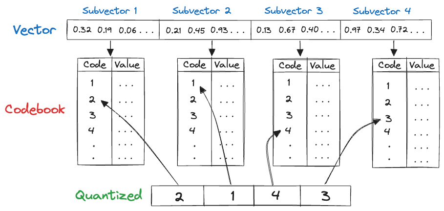

As an example, consider the above image, which visualizes quantizing a 128-dimensional vector of 32-bit integers into a 4-dimensional vector of 8-bit integers.

Original storage: 128 × 32 = 4096 bits. Quantized storage: 4 × 8 = 32 bits.In this example, quantization achieves a 128x reduction in the memory requirement of each indexed vector.

It’s important to remember that quantization is a lossy process, i.e., that no operation on the reconstructed vector can exactly recover the original vector.

Inverted File Index (IVF) Implementation

(note: acknowledge pq in here somewhere) An IVF is an index that facilitates rapid nearest neighbor searches by drastically reducing the search space. Given a large set of stored vectors, the algorithm to produce an IVF index first computes a set of centroids corresponding to an approximate solution to the

k

-means clustering problem. The centroids are then used to partition the set of vectors as follows: each vector is assigned to the centroid nearest to it in the

\ell_2

(or user-specified) metric. The set of vectors assigned to a centroid is called its cluster. This data is then recorded as an index which identifies each centroid with its cluster. The following image shows a

2

-dimensional Euclidean space partitioned according to this algorithm. The colored marks denote centroids.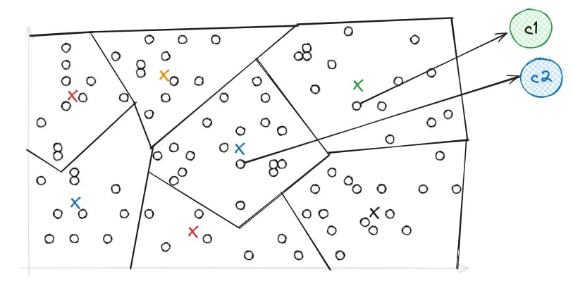

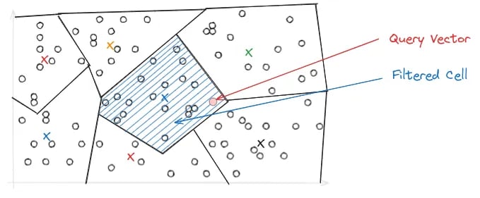
To process a nearest neighbors query, instead of a brute-force comparison of the queried vector to every stored vector, the system can instead search the much-smaller set of *centroids$ for a closest match, then execute a brute-force comparison against its associated cluster. This technique quickly eliminates the vast majority of clusters from the search space. Furthermore, since each centroid is relatively close to points in its cluster, we are likely to produce an approximately correct result. here vv During query time, depending on where the query lands in vector space, it may be close to the border of multiple Voronoi cells, which could make the top-k results ambiguous and span across multiple cells. To address this, the IVF-PQ introduces the nprobe parameter, which controls the number of Voronoi cells to search during a query. The higher the nprobe, the more accurate the results, but the slower the query.

HNSW Index Implementation

Approximate Nearest Neighbor (ANN) search is a method for finding data points near a given point in a dataset, though not always the exact nearest one. HNSW is one of the most accurate and fastest Approximate Nearest Neighbour search algorithms, It’s beneficial in high-dimensional spaces where finding the same nearest neighbor would be too slow and costly.

Types of ANN Search Algorithms

Approximate Nearest Neighbor (ANN) search is a method for finding data points near a given point in a dataset, though not always the exact nearest one. For example, HNSW is an ANN index that performs well in high-dimensional spaces where other techniques prove too slow and costly. There are three main types of ANN search algorithms:

Tree-based search algorithms: Use a tree structure to organize and store data points.
Hash-based search algorithms: Use a specialized geometric hash table to store and manage data points. These algorithms typically focus on theoretical guarantees, and don’t usually perform as well as the other approaches in practice.
Graph-based search algorithms: Use a graph structure to store data points, which can be a bit complex.

HNSW is a graph-based algorithm. All graph-based search algorithms rely on the idea of a

k

-nearest neighbor (or

k

-approximate nearest neighbor) graph, which we outline below.
HNSW also combines this with the ideas behind a classic 1-dimensional search data structure: the skip list.

Understanding $k$ -Nearest Neighbor Graphs

The

k

-nearest neighbor graph actually predates its use for ANN search. Its construction is quite simple:

Each vector in the dataset is given an associated vertex.
Each vertex has outgoing edges to its k nearest neighbors. That is, the k closest other vertices by Euclidean distance between the two corresponding vectors. This can be thought of as a “friend list” for the vertex.
For some applications (including nearest-neighbor search), the incoming edges are also added.

Eventually, it was realized that the following greedy search method over such a graph typically results in good approximate nearest neighbors:

Given a query vector, start at some fixed “entry point” vertex (e.g. the approximate center node).
Look at that vertex’s neighbors. If any of them are closer to the query vector than the current vertex, then move to that vertex.
Repeat until a local optimum is found.

The above algorithm also generalizes to e.g. top 10 approximate nearest neighbors. Computing a

k

-nearest neighbor graph is actually quite slow, taking quadratic time in the dataset size. It was quickly realized that near-identical performance can be achieved using a k-approximate nearest neighbor graph. That is, instead of obtaining the

k

-nearest neighbors for each vertex, an approximate nearest neighbor search data structure is used to build much faster.
In fact, another data structure is not needed: This can be done “incrementally”. That is, if you start with a k-ANN graph for n-1 vertices, you can extend it to a k-ANN graph for n vertices as well by using the graph to obtain the k-ANN for the new vertex. One downside of k-NN and k-ANN graphs alone is that one must typically build them with a large value of k to get decent results, resulting in a large index.

Hierarchical Navigable Small Worlds (HNSW)

HNSW builds on k-ANN in two main ways:

Instead of getting the k-approximate nearest neighbors for a large value of k, it sparsifies the k-ANN graph using a carefully chosen “edge pruning” heuristic, allowing for the number of edges per vertex to be limited to a relatively small constant.
The “entry point” vertex is chosen dynamically using a recursively constructed data structure on a subset of the data, similarly to a skip list.

This recursive structure can be thought of as separating into layers:

At the bottom-most layer, a k-ANN graph on the whole dataset is present.
At the second layer, a k-ANN graph on a fraction of the dataset (e.g. 10%) is present.
At the Lth layer, a k-ANN graph is present. It is over a (constant) fraction (e.g. 10%) of the vectors/vertices present in the L-1th layer.

Then the greedy search routine operates as follows:

At the top layer (using an arbitrary vertex as an entry point), use the greedy local search routine on the k-ANN graph to get an approximate nearest neighbor at that layer.
Using the approximate nearest neighbor found in the previous layer as an entry point, find an approximate nearest neighbor in the next layer with the same method.
Repeat until the bottom-most layer is reached. Then use the entry point to find multiple nearest neighbors (e.g. top 10).

Get started

Model training

Guides

Feature Engineering (Geneva)

Support